

By Biserka Kolarec
Students often learn a classical definition of probability early in the process of developing statistical literacy. That definition states that if there are equal odds of all experiment outcomes or events, the probability of a specific event equals the number of favorable outcomes divided by the number of all possible outcomes.
The simplest example of a classical probability experiment is a coin toss: One throws a coin and records which side shows when it lands—a head (H) or a tail (T). The sample space consists of two events {H, T}. Here, one supposes the coin is symmetrical. By the classical definition of probability, the probabilities of obtaining either the head or the tail are the same and equal to 1/2. The classical probability formula is a natural concept, and students adopt it instantly.
Since the number of all possible outcomes in the experiment of tossing one coin is small, one quickly moves to a more complex experiment of tossing more coins. Let us consider experiments of tossing two coins. Most probability books bring such experiments with no further explanation. For example, in the classical probability book A First Course in Probability, the following example is given:
If the experiment consists of flipping two coins, then the sample space consists of the following four points: S = {(H, H), (H, T), (T, H), (T, T)}
The formulation “flipping two coins” suggests two coins are thrown during one toss. Is the reasoning in such an experiment really so simple? Not quite. Students have doubts about the sample space size if told we toss two identical coins.
The Problem
Consider the experiment of tossing two identical coins in a single throw. A significant percentage of students are of the opinion that there are just three possible outcomes of this experiment. Namely, students reason one can obtain two heads (H, H), two tails (T, T), or one head and one tail (H, T). Nothing strange, since that is exactly what can be observed. Asked what the probability of obtaining one head and one tail is, students will answer it is 1/3 (one favorable out of three possible outcomes), and that complies with the classical definition of probability. Such reasoning can be enforced by posing the following ternary problem:
Consider the following experiments, and for each experiment, write down all possible outcomes, determine the number of outcomes, and determine the probability of obtaining one head and one tail.
Experiment 1: One tosses a coin twice. Denote all possible outcomes as ordered pairs (-, -), where the first entry labels the outcome of the first toss, and the second labels the outcome of the second toss.
Experiment 2: One tosses two coins of a different type during one single throw.
Experiment 3: One tosses two identical coins during one single throw.
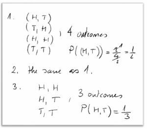
All three experiments were deliberately formulated as one problem to make students suspect their sample spaces might not be the same. Since they were given instructions for labeling outcomes, almost all students managed to recognize four possible outcomes of Experiment 1. Likewise, students concluded that if there is an agreement about the order in which one labels outcomes, there are four possible outcomes in Experiment 2, as well.
To summarize, the outcomes of the first two experiments can be written as ordered pairs: (H, H), (H, T), (T, H), and (T, T). By the classical probability definition, students concluded the probability of getting one head and one tail equals 2/4=1/2 in both experiments. Further, more than 60 percent of students wrote that all three experiments have four outcomes and probabilities of obtaining one head and one tail equal to 1/2. However, for almost 40 percent of students, the answer was as given in Figure 1.
There were two confronted groups of students with different opinions about the total number of outcomes in Experiment 3. The main question was whether we need to distinguish between experiments of tossing two different or identical coins in one throw. Students were asked to explain why they thought the total number of outcomes in Experiment 3 is three or four. They discussed the matter in small groups in the spirit of peer instruction introduced by Eric Mazur in “Peer instruction: Getting Students to Think in Class.” We did not interfere with the discussion.
In the end, the minority persuaded the majority to change their opinion! The reasoning was since there is no way to visually distinguish between the outcomes (H, T) and (T, H), there are just three outcomes one can spot. These are outcomes H-H, H-T, and T-T, and we are free not to write them anymore as ordered pairs.
In Experiment 3, students concluded there are just three outcomes and, based on the classical definition, the probability of obtaining one head and one tail is 1/3 (one favorable out of three possible outcomes). After the discussion, almost all students agreed on that.
Our goal to actively and authentically engage students in the problem was achieved. Students took responsibility for addressing the problem; it was time to guide them to where they needed to be.
Guidance to the Correct Conclusion
We did not deal with the axiomatic definition of probability, so we introduced students to three viewpoints of the probability definition. Besides the classical definition, the probability of the occurrence of an event can be viewed as the relative number of times we expect the event to occur in a large number of trials. Furthermore, one can speak of a subjective concept of probability as a measure of belief. In an experiment of a single coin toss, where there are two possible outcomes and with the logical assumption that the coin is symmetrical, all three definitions coincide. A subjective, or epistemic, interpretation of probability suggests (just like the classical one) that head and tail are equally likely to appear with the probabilities of 1/2 each. The definition through relative frequencies assumes repeating the experiment a large number of times and finding the probability of an event as a limit of the resulting ratio of the number of occurrences of an event and a number of times the experiment was performed. If one has doubts about some probability, the relative frequency approach is just a means to find out the right answer.
Students concluded there is a way to check if the probability of obtaining one head and one tail in two identical coin toss experiments equals 1/3. They experimented with tossing two identical coins a large number of times. Students were divided into pairs, and each pair counted the number of times one head and one tail appeared by tossing two identical coins 30 times. All results were unified to calculate the relative frequency of the event.
Students were surprised when it turned out to be close to 1/2, not 1/3! That observation led to the following conclusion: Even though one cannot distinguish between the outcomes H-T and T-H, they happen anyway.
In conclusion, the finding was that the sample space in the experiment of tossing two identical coins consists of four outcomes. Further, the probability of obtaining one head and one tail is twice the probability of obtaining either two heads or two tails. We noticed that both, those who were right about it and those who were wrong, seem convinced about the size of the sample space.
Discussion of the Problem
Tossing two coins is the most elementary random experiment mentioned in almost all statistical textbooks. Most textbooks assume a straightforward understanding that there are a total of four possible outcomes in experiments of tossing two coins. The authors do not comment on whether the two coins are identical.
According to the case here, students make a distinction in the size of the sample space if told one tosses two different or two identical coins. We keep confronting the same problem year by year, generation by generation: A relatively large percentage of students had an opinion that, in the experiment of tossing two identical coins, the sample space consists of just three events. Even those who thought there are four possible outcomes were not sure enough to persist in their opinion when confronted with a different one.
The lecture above that leads students to the right conclusion of the sample space size takes time a teacher may lack. It would be better to ensure no misunderstanding about the sample space in the first place. There is a simple way to do that: Speak about a coin being thrown two times. In such experiments, outcomes can legitimately be labeled as ordered pairs and students will likely have no problem writing all four down. This approach can also be found in some statistics books, for example A Modern Introduction to Probability and Statistics: Understanding Why and How.
We know from our teaching practice that students can easily generalize and calculate the number of all possible outcomes in the experiment of tossing a coin more than twice. So, in experiments that repeat n times, the total number of outcomes equals 2n. The only weakness in such experiments compared to multiple identical coin toss experiments is if actually performed, they would be more time-consuming. However, it is a small, if any, price to pay since most experiments we “perform” are performed mentally (i.e., one reasons out probable outcomes and their probabilities without actually experimenting).
The reader may object to the idea of speaking about tossing one coin twice instead of tossing two identical coins simultaneously. However, thinking about the outcomes of the experiment of flipping one coin twice can lead to a better understanding that they are the same as in the experiment of flipping two coins at the same time. Indeed, no matter if two identical coins are thrown simultaneously, likely they do not land at the very same moment. This justifies considering experiments of tossing one coin twice.