Developing the Theory of Hypothesis Testing: An Exploration
Craig Lazarski, Cary Academy
There are many concepts associated with hypothesis testing, but it all comes down to variation. How unusual is the variation we observe in a sample?
Students can often lose sight of this basic idea once they have learned the various procedures introduced in an introductory statistics course. Further, they may blindly follow the procedure and never question the impact of the sample size or magnitude of variation on the conclusion they draw.
I developed an R Shiny app inspired by a dice activity in which students try to estimate the distribution of dice produced by six companies and determine if they are fair. The app allows students to test hypotheses and provides the test statistics, p-values, and sampling distribution based on chosen sample size so they can explore the effect sample size has on p-values. It also allows students to explore the power of a test by repeatedly testing the same hypothesis with randomly sampled data and examining visual evidence of the rejection rate. Through this activity, students develop an intuitive understanding of the power of a hypothesis test and improve their understanding of how and why a hypothesis test produces results.
This task was inspired by a simple question: Can you tell if a die is fair? To anyone versed in basic statistical principles, this is a straight-forward task. You should roll the die as many times as possible, and then the law of large numbers will take over and reveal the true distribution. When students approach this task, the results can be surprising.
Day 1: Classroom Data Exploration
To explore this question, I directed students to the first page of the Shiny app. I asked each student to explore one dice manufacturing company. To start, I showed the students how to select a company and choose a sample size. Next, I asked them to describe the results presented by the app, but I did not give them further directions.
After allowing a few minutes for exploration, we came together for a joint discussion and I asked, “Who thinks they found a company that has fair dice?” One student responded that their company, High Rollers, was fair. Then I asked if anyone else in class had this company and, if so, did they come to the same conclusion? Another student responded that they found the company to be unfair.
Analyzing Student Responses for Group Discussion
When I asked the students to explain their results and how they came to their conclusions, I got the following responses:
Student 1: I set the sample size to 100 and looked at the graph. The bars were relatively close to the same heights. Then I repeated this three times and the results were similar, so I concluded the die was fair.
Figure 1: Student 1 histogram with 100 samples
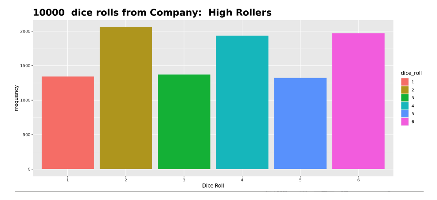
Student 2: I set the sample size to 10,000 and looked at the graph. The bars were different and, when I repeated this, it consistently showed a similar pattern each time.
Figure 2: Student 2 histogram with 10,000 samples
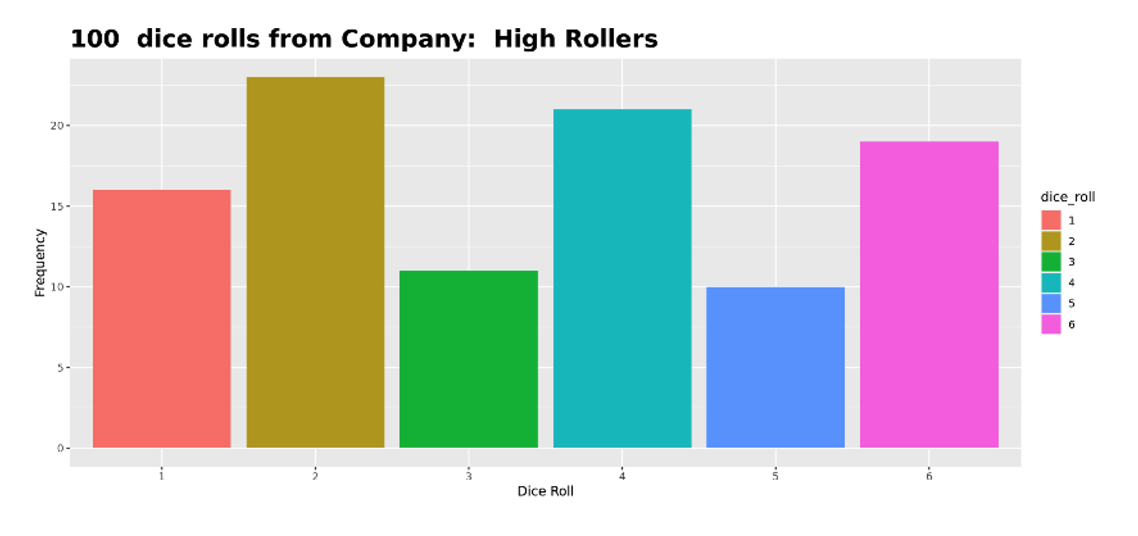
Student 1 considered the variation and believed what they were seeing was natural variation one should expect when rolling the die 100 times. Since the bars changed for each sample but the overall pattern seemed to be around a single value for each bar, they concluded it was fair.
Student 2 discovered the law of large numbers. They recognized that the results from sample to sample were very consistent and the bars were not equal. Student 1, after hearing Student 2’s explanation, quickly recanted their theory.
Once we discussed the law of large numbers in more detail, I asked again, “Who thinks they have a fair company?” Another student responded that Pips and Dots is a fair company, and they also used the law of large numbers as the basis for their conclusion. Figure 3 is a graph of 10,000 rolls of a Pips and Dots die using the simulation.
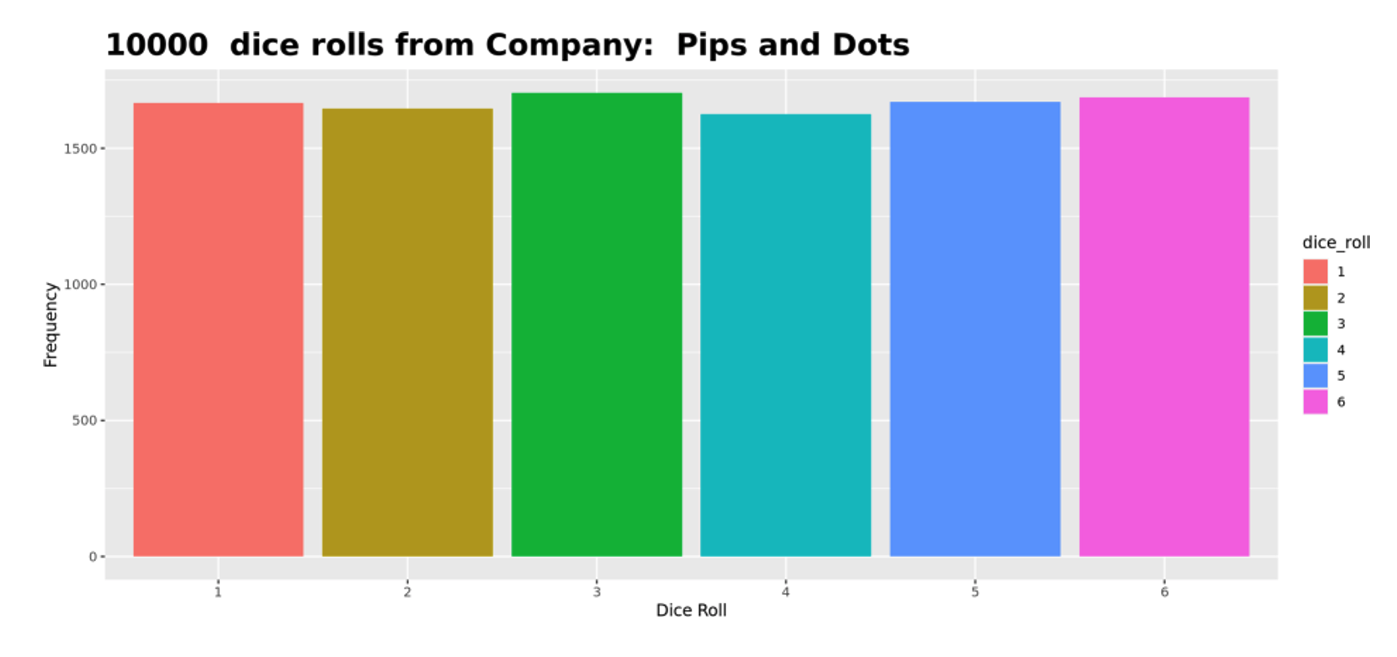
Figure 3: A graph of 10,000 rolls showing Pips and Dots is the only company with a fair distribution
The students all seemed fairly convinced that this company produced a fair die, but I asked them if they were concerned that not all the bars were exactly equal. Could it be that the die is only slightly unfair? How can we measure such deviations and decide? Essentially, I was leading my students to the need for a hypothesis test in this scenario.
We took the results above for the fair die, and I developed the goodness of fit procedure with my students. These students had already completed a lesson on one- and two-proportion z-tests, so hypothesis testing was not a new concept. Our hypothesis test led us to the correct conclusion that they were fair.
End of Day 1: Student Homework Assignment
For homework, I asked students to log in to the Shiny app from home, along with the second tab—“Chi Square Analysis”—to help them complete their homework. This second tab is an extension of the first.
Background on the Chi Square Analysis Logic and Code
Just like the first tab, I use the same distribution for each of the dice manufacturing companies throughout every tab in the app. These distributions can be configured through a simple text file, company_weights.csv, which is loaded when the Shiny app is launched.
The only options on this tab are to again select a manufacturer and to set the sample size, indicating how many rolls the student wishes to simulate. The output now includes two graphs. The first is a modified version of the histogram exactly as shown on the first tab, but it has an additional line drawn to indicate where the expected value of each die would be if the die were fair.
I added a second graph that plots the test statistic against a chi square distribution with five degrees of freedom that models the rolls of a six-sided fair die and indicates the rejection region. Now, each time the student clicks the “Update Sample Size” button, the test statistic is plotted on this second graph, allowing the students to see if it lies in the rejection region (see Figure 4).
Note that the alpha level is fixed at 0.05. Further, the actual test statistic and p-value (rounded to four decimal places) are provided under the summary information.
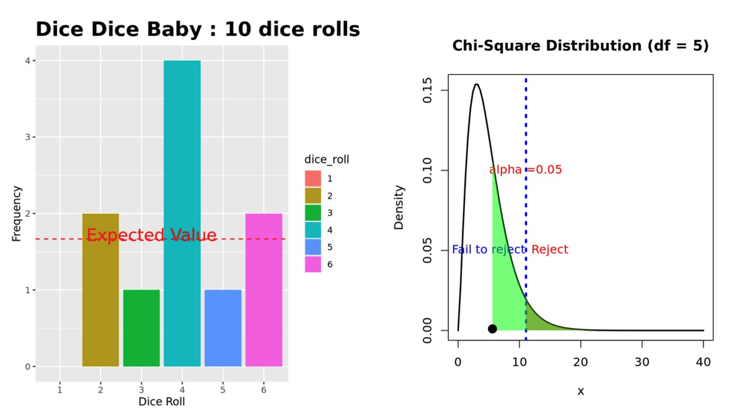
Figure 4: Example of chi square analysis plotting our test statistic
Tasks Left for Student Completion
Students were asked to respond to the following questions for this exploration:
- Do you believe the dice produced by Dice Dice Baby are fair? Without doing a goodness of fit test, what evidence is there for your conclusion?
- What is the minimum sample size that can be used to perform a goodness of fit test for this company if we want to ensure the expected counts are at least 5?
- Use the app to generate a sample using the minimum sample size and conduct a goodness of fit test.
- Use the app to generate a sample of 600. Conduct a goodness of fit test using this data.
- The Dice Dice Baby company is not producing fair dice. Go to the second tab on the app, “Chi-Square Analysis.” Using the Dice Dice Baby company, run several tests using a sample size of 30 and note the p-value and conclusion you would make. (You will find the test statistic and p-value under the frequency table.) Repeat using a sample size of 600 and note the p-value and conclusion you would make. Make a conjecture about the role sample size plays in a hypothesis test.
- Use the app to determine what minimum sample size is necessary so the test concludes that the dice is not reliably fair. Reliably means that, in most cases, the test will correctly determine the dice are unfair.
These questions asked students to perform a goodness of fit test on a company they thought to be unfair. Using a small sample size, the student should reach a fail to reject conclusion, while a large sample size would lead them to reject. Using the app, the students are able to quickly execute many iterations of this activity to ensure the response they are seeing isn’t a fluke.
Sample Responses from Homework Task
Question 5 asks students to explain what they observed. Sample responses include the following:
Student 1
“The smaller the sample size, the larger the p-value and therefore the more likely it is we would fail to reject the null hypothesis of each face being rolled equally. The larger the sample size, the smaller the p-value and the more likely we will reject the null hypothesis.”Student 2
“I believe that the greater the sample size, the more ‘consistency’ there will be in p-values within samples.”Student 3
“The smaller the sample size, the more scattered and unreliable the results are in a hypothesis test.”Student 4
“According to these tests, a greater sample size is more likely to produce accurate and precise results, which would help with the certainty with which we can claim to reject or fail to reject the null hypothesis.”
The responses indicate the students were developing an understanding that a hypothesis test is not infallible. They were seeing that the sample size has a direct effect on a test correctly identifying a false null hypothesis. Essentially, I took away their blind faith in hypothesis testing. Simply reaching a conclusion does not mean the student has reached the correct conclusion.
The misconception that a hypothesis test always provides the correct conclusion is a vital one to correct, and this interactive, visual exploration of test statistics makes that readily apparent to the student.
Task 3: Power of Tests
In the “Power” tab of the Shiny app is the third and final task for the students to complete. This task can be explored after an in-class discussion with the students about their homework in the previous section. The goal of this task is to restore the students’ faith in hypothesis testing by exploring the power of a test.
To begin, the students will again select a manufacturing company, choose a sample size, and perform a set number of hypothesis tests (number of simulations). Since the students have already explored the underlying distribution of the manufactures in the first two tasks, I gave them the true distribution of each manufacture just below the button “Update Sample Size.” As students change the manufacture in the drop-down selector, the true distribution is automatically updated and shown below on the left panel.
After some manual exploration, I decided to set the initial sample size to 10 and the number of simulations to 100. These parameters are intentionally not large enough to show the true power of the hypothesis test, and it is up to the students to adjust the numbers until they reach their own conclusions about the power of the test.
Just like tab two, we displayed the computed test statistics using a dot plot; however, the graph no longer had the chi square distribution overlaid as it was on the homework task.
After students clicked the “Update Sample Size” button, a distribution of the test statistics for the number of tests was displayed. The distribution was separated by a reject region that indicated those test statistics that would lead to a conclusion of reject versus those that would lead to a fail to reject conclusion. An example using dice from Dice Dice Baby with a sample size of 100 and running 100 simulations is shown in Figure 5.
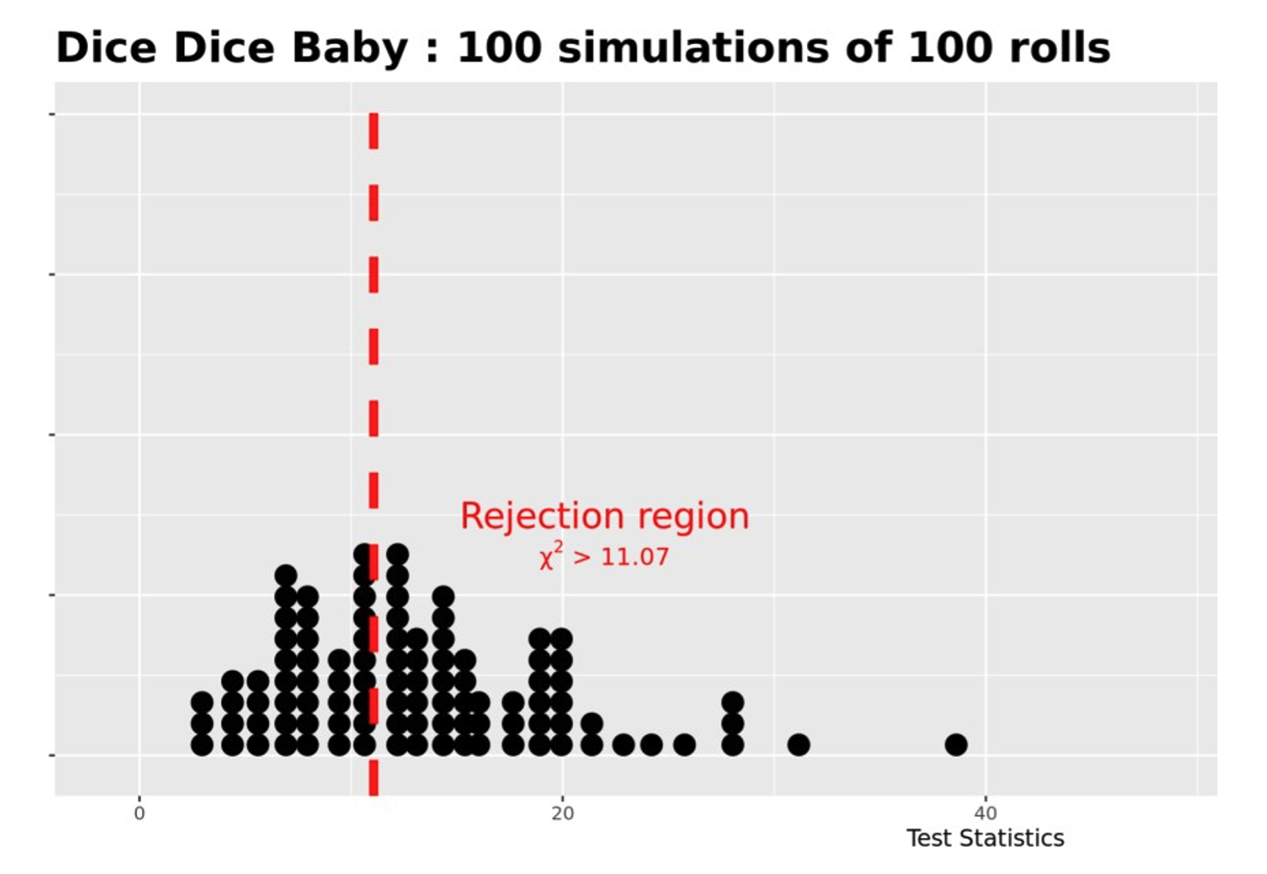
Figure 5: Power of a test example
Below this graph, I also presented students with the Type 2 error and power rate (see Figure 6) in the Shiny app.
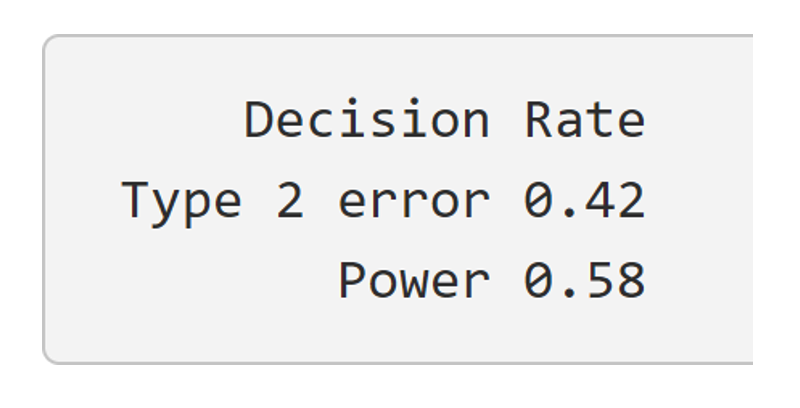
Figure 6: Power decision rates
The power was calculated as the number of observed test statistics that led to rejecting the null hypothesis out of the total number of simulations run.
Power Analysis: Guided Activity
Prior to starting the power tasks, I asked the students if they found anything strange or unexpected from their homework exploration in Task 2. One student responded that they had. The student explained that the hypothesis did not always reject when it should and changing the sample size helped. When the sample size was increased, the test more consistently rejected.
After the discussion, I asked students to work in small groups through the Task 3 activity on the “Power” tab and try to answer all the questions. As they worked collaboratively, I walked around listening and observing their work. I noted students were quickly developing an understanding of the power of a test and what a type II error was. Following are one group of students’ responses:
Dice R Us is a company close to being fair. What size sample is needed for the power to be near 90 percent?
The power is near 90 percent around 575 rolls for Dice R Us.
Dice Dice Baby is a company that is far from being fair. What size sample is needed for the power to be near 90 percent?
The power is near 90 percent around 200 rolls for Dice Dice Baby.
For the two companies you just explored, how is the sample size related to the power of the test?
For both companies that were just explored, the power of the test increases with sample size.
How is the degree to which the truth varies from the null hypothesis related to the power of the test?
If the truth is far from the null hypothesis, the power will be much higher, as it will be easier for the test to reject the null hypothesis.
Type II error is also presented. What is its relation to power? Can you explain what a type II error is?
Type II error is the opposite of power, meaning it’s the proportion of simulations that failed to reject the null hypothesis even when it was false.
The students above are clearly showing a deep understanding of both power and type II errors. They understand the role sample size has, as well as the magnitude of the difference from the null hypothesis.
After the exploration, we discussed the answers to the above questions as a class and students showed similar understanding.
Finally, we addressed group responses to the last question in this task, which asks:
Pips and Dots is a company that produced fair dice. Evaluate the power of the test for this company? Can you explain what you are seeing?
The purpose of this question is to challenge students’ understanding of everything they just demonstrated in their prior exploration. The company being analyzed, Pips and Dots, is the company that produced fair dice. Therefore, the test should never reject and, in theory, the question of power is irrelevant.
However, the app still generated a value for power as shown in Figure 7.
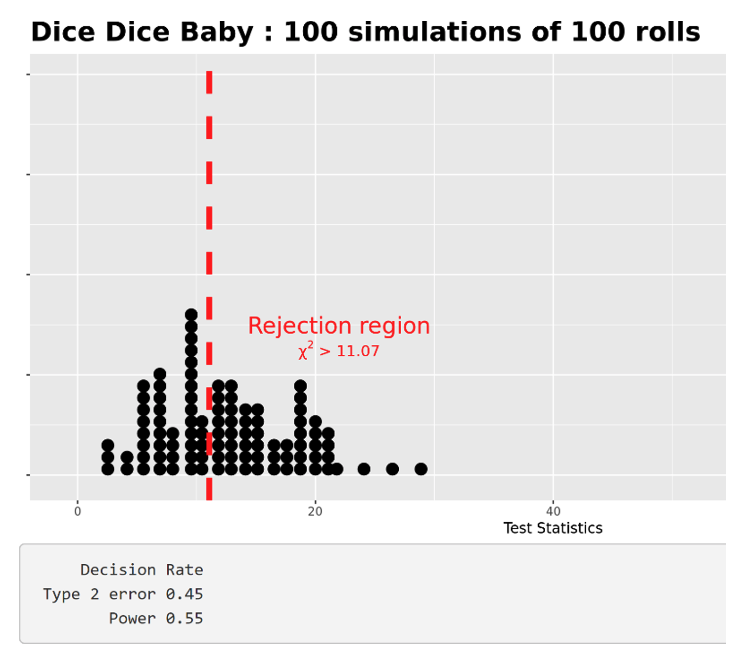
Figure 7: Test statistics of the “fair dice” company
Following are examples of the students’ responses to this question:
Group 1
Since the dice were fair, the power is very low, as it is much harder to reject a null hypothesis that is correct.Group 2
The power is extremely low and, as the sample size increases, the power only gets lower because when a company is fair, the company should not reject the null, and the power is the chance that it will correctly reject the null.Group 3
The power stays low even when the sample size is high. The reason it stays low is because why would you reject a correct null?
These responses led to a discussion about the nuance of power in which I specified that we only calculate the power of a test for specific alternatives. When we assume the null is false, we then attempt to determine what the chance is that our test will catch it.
Students understood the power was irrelevant in this case. Even more impressive, a few students recognized the power was describing a mistake. The power was calculating how often the test incorrectly rejected a true null hypothesis, which is similar to a type I error.
It was important that I noted the power calculated was not a type I error, but the connection they made cemented their understanding of the three elements used to evaluate the quality of a hypothesis test.
Personally, my understanding was also affected. One student asked if this was related to the confidence level when constructing a confidence interval. I had never made this connection before, and it is absolutely true! Just as the confidence level evaluates how often an interval will capture a parameter, the power of a test evaluates how often a hypothesis test will correctly reject a false null.
My conclusion after completing this activity is that the students developed an intuitive understanding of what it means to have a test with high power and the types of mistakes that are possible when completing any hypothesis test.
In the past, I have observed students could often parrot back the technical definitions but had trouble interpreting them in their proper context. After completing this activity, students were able to easily identify errors in context, in addition to the power of a test. And they demonstrated an ability to think more critically about the procedures they were employing.