
Model t, or a Newer Randomization?

Sean Bradley
Anyone who loves math appreciates a good mathematical model. There is no shortage of useful workhorses in statistics–normal, t, F, and chi-square distributions come quickly to mind.
Mathematicians and statisticians of yesteryear developed these beautiful models to overcome the inability to use brute force methods to answer statistical questions. For example, when R. A. Fisher invented his randomization techniques, he had to resort to theoretical probabilities by way of binomial and multinomial distributions.
For the general student in her first (and perhaps only) statistics course, however, these models seem to come out of nowhere and usually with no plausible justification except that “they work.” Because of this, teaching such models can hinder student understanding by obscuring the key to what makes statistical methods work: randomness and probability.
Today, computing power is cheap and accessible, so past models are not the only option for introducing students to these ideas. We want to make the case that randomization techniques could replace the mathematical models we have relied upon for so long–at least in introductory statistics. Randomization techniques are pedagogically superior, easy to understand, and easily transferable.
An Illustration
Before making the case for using such techniques in an introductory or Advanced Placement course, consider an example found in The Statistical Sleuth.
Example 1
Investigators randomly assigned laboratory guinea pigs to one of two groups–one dosed with tuberculosis bacilli and the other a control group. They recorded the lifespan of each guinea pig, a quantitative variable measured in days from birth, as the main outcome.
Dotplots and boxplots of the data reveal differences. Lifetimes in the bacilli group tended to be shorter and displayed less variation than the control group. The dotplot for the control group raised a question of bimodality (an observation that experts are likely better able to clarify). The lifespans of guinea pigs treated with bacilli display a marked right skew, with a couple long-lived outliers. It seems there is something different in the groups of guinea pigs. Hence, the question: Do treated guinea pigs tend to live for a shorter number of days?
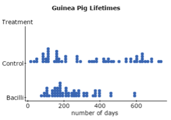
Display 1 Dotplots of lifetimes (StatCrunch)
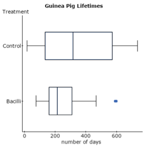
Display 2 Boxplots of lifetimes (StatCrunch)
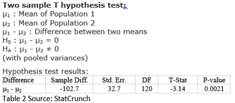
The strategy for answering this question is easy to explain. In the randomized sample, the difference in means turned out to be about 103 days. This seems large, but remember sampling variability. We must learn how common it would be for random assignments to two groups, after the fact and independent of the treatment, to reproduce a difference at least this large. If such a difference is common, then randomness could be the culprit for the difference in means. Otherwise, we will have evidence that the bacilli treatment is responsible, especially in light of the experimental design.
A t-Test
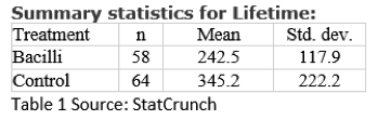
For students who learn a traditional t-test, will this strategy be evident? Experienced statisticians and teachers know neither the data nor a graphical exploration are necessary for a bare-bones t-test. We need only the summary statistics in Table 1 to compute a p-value and determine whether there is a statistically significant difference.
Many students would see this simple pathway to “an answer” as an advantage to a t-test, but teachers know the importance of exploring the data (both graphically and numerically) and considering study design. The goal is to learn about guinea pigs, not just acquire a p-value!
Teachers know, too, that a t-test requires checking certain assumptions (i.e., sample sizes, distribution shapes, and random assignment). At the introductory level, these criteria can seem artificial to students, and it is no surprise if they choose to avoid them. After all, a student might wonder, what do the criteria have to do with the p-value or our strategy?
A Randomization Test
Now consider a randomization test using free web-based StatKey software. This test will make the strategy we laid out above, to determine if a difference in means at least as large as 103 days could be due to random chance, completely transparent. The idea is to re-shuffle the guinea pig lifespan values into two groups many times, and then see how often a difference in means at least as large as 103 days occurs. This is what a t-distribution models, but a randomization test just does it! We do not need any model, since StatKey will create a dotplot that shows the results of thousands of randomizations.
Once we upload the data, StatKey is ready to go. Here is a two-minute YouTube video that shows how to create the randomization test.
The first pedagogical “bonus” of this technique is that it requires the actual data. A mere summary of sample sizes, means, and standard deviations is not enough. This physical connection to the data–and not just the summary–makes it easier to convey the message that we begin with data exploration.
Another advantage is that StatKey allows us to begin creating randomizations one at a time. Display 3 shows the differences in means for only the first 10 randomizations. Beginning “slowly” helps facilitate a discussion of the nature of randomization distributions; we can explain to students that each dot conveys the difference in means for a single random re-shuffle. The next step is to follow up with a question: “Why aren’t all the sample differences equal?” Randomness is a key (and visual) aspect of the test, right in front of us!
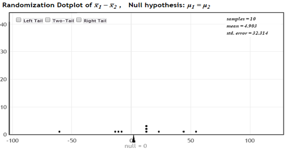
Display 3 Dotplot with 10 StatKey randomizations
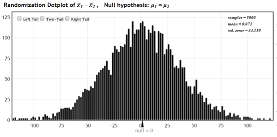
Display 4 Dotplot with 5010 StatKey randomizations
Next, we quickly and easily create several thousand randomizations. We prefer a minimum of 5000, and Display 4 shows the results of the original 10 randomizations along with 5000 new ones. Even without checking the p-value, it is obvious a sample difference of 103 days would be highly unlikely to occur by chance alone. There must be something else going on.
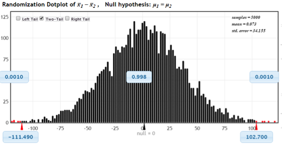
Display 5 Randomization distribution displaying P ≈ 0.001 + 0.001.
The p-value, however, is right before our very eyes. Using the “two-tail” option, Display 5 shows those dots from the randomizations “at least as extreme as the one in the sample” colored red, and the computed proportion of these extreme values among all the 5010 randomizations (p-value ≈ 0.001 + 0.001 = 0.002 for this example).
Observations
This example allows consideration of a few natural items worthy of a teacher’s consideration.
First, some students might be confused if the person next to them has a (slightly) different p-value. They often know randomness is responsible, but need to be reassured it is okay. We point out that even with these small differences in p-value, the conclusion (reject the null hypothesis) will be the same.
Second, p-value from a randomization test and a traditional t-test are unlikely to be equal. This reveals a point often obscured by black-box t-tests: All p-values are estimates. Since t-test software will yield the same p-value every time we run the data, it can be easy for students to forget the t-distribution is a model that provides an approximate p-value. The approximate nature of p-values is more obvious with randomization testing, since its p-values will vary for different tests on the same data.
A third point is more subtle. The null hypothesis H0: µ1 = µ2 mentions only population means. It does not explicitly refer to sample sizes, standard deviations, shapes, outliers, or other attributes of the data. But an honest t-test requires checking sample sizes (n = 30 is often the “magic number”), deciding whether to use pooled or unpooled samples to estimate standard deviations, and checking shapes and outliers for the sample distributions, perhaps even assuming the underlying populations are normal. Considering these limitations, teachers will appreciate two advantages of randomization tests:
- Since a randomization test does not rely on the limiting behavior of a theoretical model, it does not need any of these assumptions.
- All the features of the samples’ distributions (i.e., shapes, spreads, outliers, etc.) are built into the randomization process.
Indeed, a randomization test does not model a sampling distribution in some ideal sense, but uses the nitty gritty data values themselves to produce the simulated distribution–all the data, every time. It is easy to prefer the randomization test’s transparency and simplicity. It is a test without guile.
Finally, we mention an important point made by Cobb. The simulated randomizations mimic the randomization of the guinea pigs at the start of the study. Thus, there is a strong and natural connection between study design and the statistical method used to investigate the results. We simulate randomizing the data values to learn about the possible effects of the initial randomization.
Study Designs
Our guinea pig example uses the best kind of study design–a randomized comparative experiment. What about observational studies? Whenever we compare two groups, if the question is, “Could random assignment explain the differences we see, or is there something else going on?” then randomization testing works. Consider two more examples.
Example 2
In 1898, a severe winter storm struck Providence, Rhode Island. People brought a number of freezing sparrows to the laboratory of Hermon Bumpus, a Brown University professor. Some died, others survived. Bumpus took advantage of the opportunity to conduct an observational study, comparing the average lengths of sparrows that died with those that survived.
The sparrows were a sort of representative sample of the local sparrows at that time. In other words, nature drew two samples from a single population. From the statistical point of view, Bumpus needed to decide whether the sparrows got into the two groups at random, or if there was something else going on. A randomization test could reveal which makes more sense.
Example 3
Consider the wage gap between women and men in the United States. We might undertake an observational study to determine if there is a difference in average earnings in a particular profession. To do so, we would compare average salaries for samples from two distinct populations–women and men. The question is, “Could such a difference occur by chance if we had chosen the two samples independent of sex?” Again, a randomization test could rule this out.
Generalizing to Other Tests
The two-sample randomization test for comparing means has counterparts in other statistical testing. For example, the idea for comparing two proportions is identical to the approach we have described. There are also randomization approaches to one-sample hypothesis testing, confidence intervals, correlation, and regression. (We list several introductory textbooks later that take varying approaches.)
Moreover, comparisons among three or more groups require only that we show students how to compute a useful test statistic to use in the randomization. In fact, the test statistics can be quite simple. For example, there is no need for a chi-square test statistic to perform a comparison of multiple proportions. Absolute deviations work for randomizations and have the advantage of being intuitive.
In any of these situations, the strategy is to do the following:
- Create a test statistic that measures how far the data are from what a null hypothesis predicts (perhaps equal means or proportions)
- Simulate thousands of values of the test statistic via a randomization process
- Estimate a p-value by counting how often a sample allotment at least as extreme as the sample’s occurs
This extension of the basic idea of two-sample randomization testing is simple, appealing, and makes intuitive sense to students.
Eliminate the t-Test?
Teachers of introductory statistics courses are not always in control of curriculum. For example, what about those preparing students to take an Advanced Placement test, which includes t-tests as the method of choice for exploring the difference between two means? Should AP teachers include randomization techniques? A related question a teacher might ask is, “Since my students will encounter t-tests after they leave the classroom, don’t they need to learn about them?”
These are important questions. At the very least, if randomization testing leads to clearer and deeper understanding of p-values, then it seems important to include it in an introductory course. When we begin with t-tests, students tend to lose the core ideas in a morass of models, assumptions, and details. Would it be better to first lay the foundation of randomization testing as a way to understand the role of randomness in statistical testing? Then one can explain the role of models in testing.
Conclusion
I mentioned earlier that randomization testing is featured in several prominent texts. The ones I have seen still include theoretical models; they have served us well and provide valuable insight into many key facets of statistics. I do question, however, their usefulness in a first course that might be the students’ only statistics course. Perhaps it is better to investigate these models more in depth after an AP or introductory statistics course.
Textbooks for introductory courses that use randomization techniques include the following:
- Lock, Robin H. et al. 2013. Statistics: Unlocking the Power of Data. Wiley.
- Rossman, Allan J., and Beth L. Chance. 2012. Workshop Statistics. 4th ed. Wiley.
- Tintle, Nathan et al. 2014. Introduction to Statistical Investigations. Wiley.
Author:
Sean Bradley
Clarke University
Dubuque, Iowa
Further Reading
- Doksum, K. 1974. Empirical probability plots and statistical inference for nonlinear models in the two-sample case.” Annals of Statistics 2 p. 274. We learned of this in Ramsey and Schafer, The statistical sleuth, 1997, Thomson Publishing, p. 49.
- StatKey is freely available and accompanies the textbook by Lock et al., which has many good examples, ideas for lessons, and discussions about randomization techniques. StatCrunch also contains randomization tools, but is a subscription service.
- Cobb, G. 2007. The introductory statistics course: A Ptolemaic curriculum?” Technology Innovations in Statistics Education.
- The data are at the Field Museum website in an online article by Peter Lowther. We learned of this data in Rossman and Chance, Workshop Statistics (4E), 2012, Wiley & Sons Publishing, p. 198.